Project Overview & Abstract
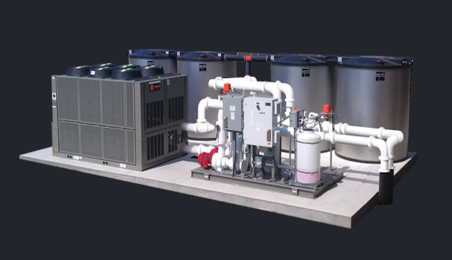
This project for MECH 4420, “Project 3,” focused on addressing the significant increase in cooling load for a large athletic facility undergoing expansion. The HVAC system required substantial upgrades, including an additional chiller. The core objective was to identify the most cost-effective design configuration for adding an Ice Thermal Energy Storage (TES) system to be used during peak hours. Four design alternatives were evaluated. The study concluded that “Alternative 4,” despite having the highest initial capital cost, would offer the shortest payback period due to significant annual operational savings.
I. Introduction and Problem Definition
As the athletic facility planned for expansion, its existing HVAC system, comprising two 1300-ton electric centrifugal chillers, would become insufficient. An additional 1300-ton chiller was deemed necessary regardless of other upgrades. This project specifically evaluated the integration of an Ice Thermal Energy Storage (TES) system. Four distinct design configurations for the TES system and chiller operation were analyzed to determine the optimal solution based on:
- Increasing overall CHW (Chilled Water) plant capacity.
- Future-proofing for subsequent cooling load increases while reducing peak electric power demand.
- Providing the best viable energy cost savings.
II. Givens, Assumptions, and Core Calculations
The analysis was based on defined financial and operational parameters:
Key Parameters:
- Time-of-Use (TOU) Electric Rates:
- On-peak (1:00 pm – 5:00 pm): $0.3/kWh
- Mid-peak (10:00am – 1:00 pm & 5:00 pm - 10:00 pm): $0.19/kWh
- Off-peak (10:00 pm - 10:00 am): $0.15/kWh
- Capital Costs:
- Conventional electric chiller plant: $1800/ton
- Ice-making chiller plant: $800/ton
- Ice TES storage: $500/ton-hour
- Operating Efficiencies:
- Conventional electric chiller plant EER: 11 (COP = 3.22)
- Ice-making chiller EER: 16 (COP = 4.69)
Core Formulas:
Operating Cost (OC) = Energy Consumption * TOU RatekWh = (Load (tons) * 12) / EEROverall System Capital Cost = (Max System Outputs * Price) + (TES Capacity * Price)Savings = Base Operation Cost - Alternative Operation Cost
III. Design Alternatives & Analysis (Focus on Alternative 4)
While four alternatives were considered, “Alternative 4” emerged as the most promising. This alternative implemented a full storage strategy:
- The less efficient Centrifugal chiller was turned off during on-peak hours.
- The ice-making chiller’s output was increased.
- The Ice TES system capacity was expanded to cover peak loads. The premise was that higher initial capital investment would be offset by substantial annual savings from shifting energy consumption to off-peak hours for ice generation, leading to a quicker payback.
Table 5 (from PDF Page 4): Key Thermal Calculations for Alternative 4 (Selected Hours)
| Hour Starting | Cooling Load (tons) | Centrifugal Output (tons) | Ice TES Capacity (ton-hours) | Mode | Operation Cost ($) |
|---|---|---|---|---|---|
| 12:00 AM | 1,029.00 | 1,029.00 | 2,696.25 | charge | 218.94 |
| 6:00 AM | 1,204.00 | 1,204.00 | 5,392.50 | charge | 247.57 |
| 12:00 PM | 2,521.00 | 2,521.00 | 8,088.75 | charge | 586.57 |
| 1:00 PM | 2,675.00 | 0.00 | 8,538.13 | Discharge | 101.11 |
| 2:00 PM | 2,740.00 | 0.00 | 8,987.50 | Discharge | 101.11 |
| 3:00 PM | 2,740.00 | 0.00 | 9,436.88 | Discharge | 101.11 |
| 4:00 PM | 2,630.00 | 0.00 | 9,886.25 | Discharge | 101.11 |
| 5:00 PM | 2,445.00 | 2,445.00 | 10,335.63 | charge | 570.82 |
| 10:00 PM | 1,617.00 | 1,617.00 | 1,797.50 | charge | 315.15 |
| Total Daily | 41,970.00 | 31,185.00 | 7,374.44 |
IV. Economic Evaluation & Payback Period
The core of the economic evaluation was determining the payback period for each alternative.
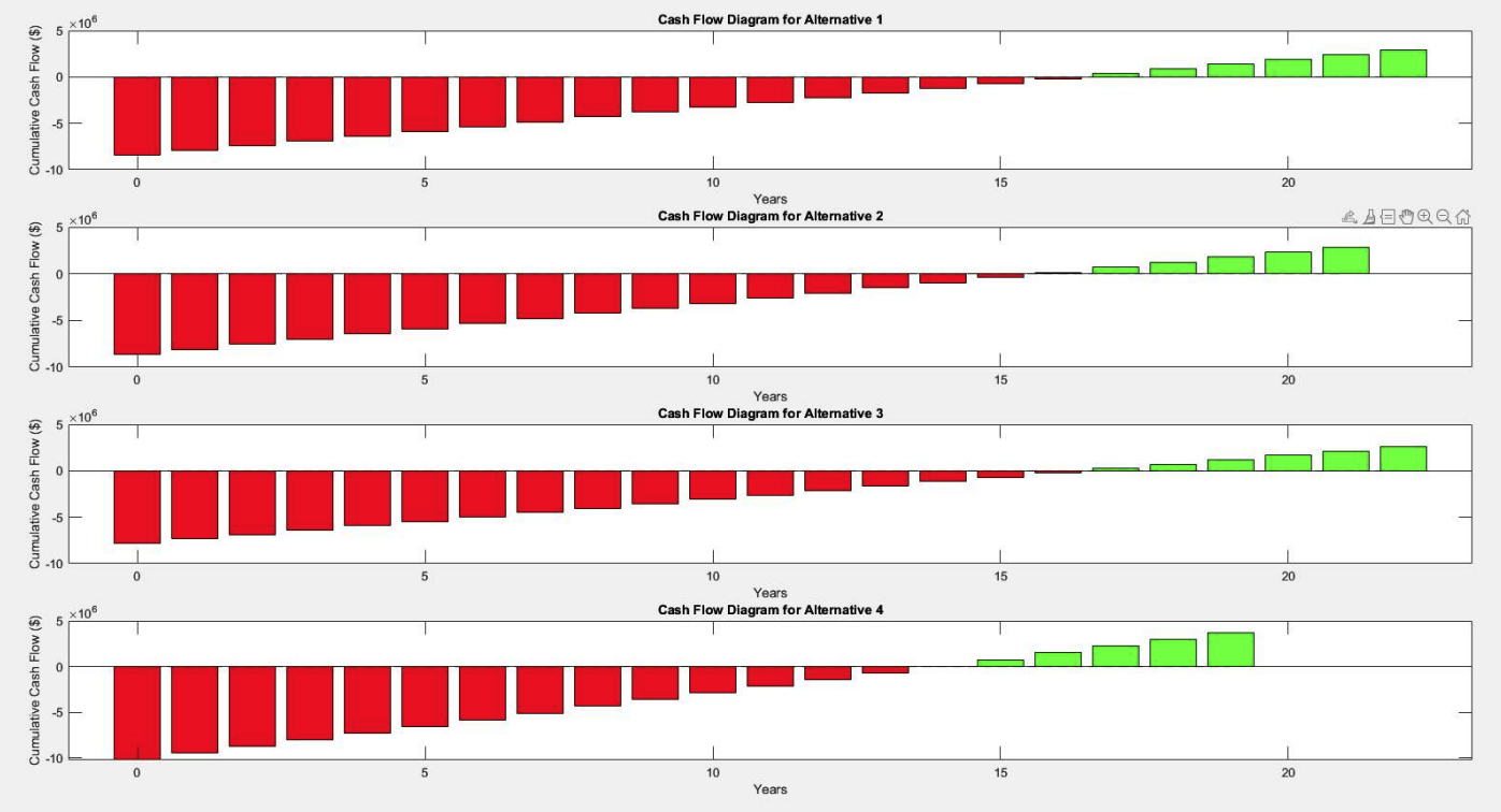
Figure 1: Bar Cash Flow Diagrams. These charts visually represent the cumulative cash flow for each alternative year-over-year, with the initial negative bar indicating capital cost and subsequent bars showing the impact of annual savings.
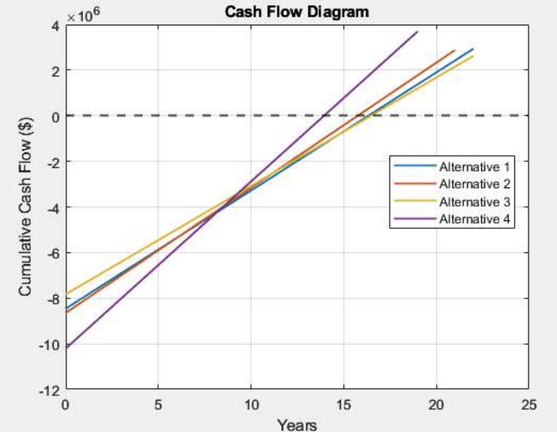
Figure 2: Linear Cash Flow Diagram. This graph plots the cumulative cash flow over 25 years for all four alternatives, clearly showing Alternative 4 achieving payback (crossing the $0 line) earliest despite its higher initial investment.
Table: Economical Analysis Summary
| System | Capital Cost | Op. Cost/Year | Savings/Year | Payback (years) |
|---|---|---|---|---|
| Base | $4,680,000.00 | $3,423,953.51 | $0.00 | 0.00 |
| Alternative 1 | $8,460,000.00 | $2,905,869.19 | $518,084.32 | 16.33 |
| Alternative 2 | $8,647,200.00 | $2,875,209.19 | $548,744.32 | 15.76 |
| Alternative 3 | $7,831,600.00 | $2,948,541.34 | $475,412.17 | 16.47 |
| Alternative 4 | $10,207,312.50 | $2,691,670.39 | $732,283.12 | 13.94 |
Results Discussion: Alternative 3 had the lowest initial capital cost but resulted in the longest payback period due to higher operating expenses. Alternatives 1 and 2 had comparable capital costs. Although Alternative 4 had the highest initial capital cost (over $10 million), its significantly lower annual operating cost led to the most substantial annual savings ($732,283.12). This allowed it to rapidly outperform other alternatives, achieving payback in 13.94 years, approximately 1 year and 10 months sooner than the next best option.
V. MATLAB Implementation for Analysis
A MATLAB script was developed to automate the calculation of payback periods and generate the cash flow diagrams. This involved:
- Defining capital costs and fixed annual positive cash flows (savings) for each alternative.
- Looping through each scenario to calculate year-by-year cumulative cash flow.
- Using linear interpolation to determine the precise payback period.
- Plotting both bar and linear cash flow diagrams for visualization.
% Excerpt: MATLAB code for payback calculation and plotting

% Parameters for 4 alternatives
capital_costs = [-8460000, -8647200, -7831600, -10207312.5]; % Initial capital costs
fixed_positive_cash_flows = [518084.3182, 548744.3182, 475412.1682, 732283.1165]; % Annual savings

num_alternatives = numel(capital_costs);
payback_periods = zeros(1, num_alternatives);
cash_flows_history = cell(1, num_alternatives); % To store yearly cash flows for plotting

% Loop through all scenarios to calculate payback and store cash flow history
for i = 1:num_alternatives
    cumulative_cash_flow = capital_costs(i);
    % Extend cash flow calculations for an additional 5 years after anticipated payback for plotting
    % (Assuming max payback around 20 years for plotting up to 25 years)
    num_years_to_plot = 25; % Max years for plotting
    current_cash_flow_path = zeros(1, num_years_to_plot + 1); % year 0 to year N
    current_cash_flow_path(1) = cumulative_cash_flow;

    year_int = 0; % Integer year counter

    % Calculate cumulative cash flow until it becomes positive
    while cumulative_cash_flow < 0 && year_int < num_years_to_plot
        year_int = year_int + 1;
        cumulative_cash_flow = cumulative_cash_flow + fixed_positive_cash_flows(i);
        current_cash_flow_path(year_int + 1) = cumulative_cash_flow;
    end

    % Fill remaining years for plotting if payback is met early
    for k = (year_int + 1) : num_years_to_plot
        cumulative_cash_flow = cumulative_cash_flow + fixed_positive_cash_flows(i);
        current_cash_flow_path(k + 1) = cumulative_cash_flow;
    end

    cash_flows_history{i} = current_cash_flow_path;

    % Linear interpolation for exact payback period
    % Ensure we don't use a zero divisor if payback is immediate or never within one year
    if year_int > 0 && (current_cash_flow_path(year_int + 1) - current_cash_flow_path(year_int)) ~= 0
        payback_periods(i) = (year_int - 1) - current_cash_flow_path(year_int) / (current_cash_flow_path(year_int + 1) - current_cash_flow_path(year_int));
    elseif cumulative_cash_flow >= 0 && year_int == 0 % Payback in year 0 (e.g. no capital cost)
        payback_periods(i) = 0;
    else % Did not reach payback or edge case
        payback_periods(i) = NaN; % Or handle as appropriate
    end

    fprintf('The payback period for alternative %d is %.3f years.\n', i, payback_periods(i));
end

% Plot the combined linear cash flow diagrams (Figure 2 from PDF)
figure;
hold on;
years_axis = 0:num_years_to_plot;
for i = 1:num_alternatives
    plot(years_axis, cash_flows_history{i} / 1e6, 'LineWidth', 1.4, ...
         'DisplayName', sprintf('Alternative %d', i));
end
hold off;
xlabel('Years');
ylabel('Cumulative Cash Flow ($ x 10^6)');
title('Cash Flow Diagram');
legend('show', 'Location', 'southeast');
grid on;
yline(0, 'k--', 'LineWidth', 1.5, 'HandleVisibility', 'off'); % Horizontal line at y=0

% Plot the individual bar cash flow diagrams (Figure 1 from PDF)
figure;
ax = gobjects(num_alternatives, 1); % Store axes handles
for i = 1:num_alternatives
    ax(i) = subplot(num_alternatives, 1, i);

    % Create year-by-year cash flows (not cumulative for bars, except year 0)
    yearly_flows = zeros(1, num_years_to_plot + 1);
    yearly_flows(1) = capital_costs(i); % Year 0 is capital cost
    for j = 1:num_years_to_plot
        yearly_flows(j+1) = fixed_positive_cash_flows(i);
    end

    % For bar chart visualization, we often show initial cost then annual savings
    % The PDF shows cumulative bars. To replicate that effect with 'bar':
    cumulative_for_bar = cash_flows_history{i};

    % Separate positive and negative parts of CUMULATIVE flow for coloring
    positive_cumulative_cash_flows = max(0, cumulative_for_bar);
    negative_cumulative_cash_flows = min(0, cumulative_for_bar);

    bar(years_axis, negative_cumulative_cash_flows / 1e6, 'FaceColor', 'r', 'EdgeColor', 'none');
    hold on;
    bar(years_axis, positive_cumulative_cash_flows / 1e6, 'FaceColor', 'g', 'EdgeColor', 'none');

    plot([years_axis(1), years_axis(end)], [0, 0], 'k--'); % Add zero line
    hold off;

    %ylabel('Cumulative Cash Flow ($ x 10^6)'); % y-label for each subplot
    title(sprintf('Cash Flow Diagram for Alternative %d', i));
    if i == num_alternatives
        xlabel('Years'); % x-label only on the last subplot
    end
    ylim([min(capital_costs)/1e6 * 1.1, max(max([cash_flows_history{:}]))/1e6 * 1.1 ]); % Consistent y-axis
end
linkaxes(ax, 'x'); % Link x-axes of all subplots
sgtitle('Cumulative Cash Flow by Year for Each Alternative'); % Super title for the figure
MATLAB code streamlined the repetitive calculations and provided clear graphical outputs for comparing the alternatives, including the generation of both linear and bar-style cumulative cash flow diagrams.*
VI. Summary and Conclusion
This project successfully identified the most cost-effective HVAC upgrade strategy for the expanding athletic facility by incorporating an Ice Thermal Energy Storage (TES) system. By evaluating four design alternatives, considering cooling requirements, capital costs, operational savings, and payback periods, Alternative 4 was determined to be the superior choice. Its full storage strategy, involving shutting down the less efficient chiller during on-peak hours and leveraging an expanded ice-making chiller and TES capacity, yielded the shortest payback period of 13.939 years, despite its higher initial investment. This demonstrates that a well-designed TES system can provide a cost-effective, long-term solution for managing increased cooling loads and reducing peak energy demand.
Key Skills Demonstrated:
- HVAC System Design & Analysis: Understanding chillers, cooling loads, TES systems, EER/COP.
- Engineering Economics: Capital budgeting, operating cost analysis, payback period calculation, cash flow analysis.
- Data Analysis & Modeling: Processing operational data and financial parameters.
- Programming (MATLAB): Automating calculations and generating visualizations.
- Problem Solving: Developing and comparing multiple solutions to complex engineering challenges.
- Technical Reporting: Clearly presenting methodology, results, and conclusions.